14  Conventions and Style

Why names (and style) are part of your statistical method

14.1 Why you should care (even if you “just want to model stuff”)

Naming conventions and coding style are not decoration. They are infrastructure.

If your names are inconsistent, your code becomes harder to read, harder to debug, and harder to share—especially once your project grows beyond “one file, one afternoon.”

“It’s the hardest job to come up with new and unique names for a variable every time you create one but this is the difference between an average programmer and a good one.”
— Vikram Singh Rawat

In scientific workflows, this difference is not about elegance. It is about traceability.

A workflow that depends on unstable or unclear names cannot be audited, reused, or trusted.

NoteThe three scientific costs of sloppy naming

• Interoperability cost:
  Non-standard names break workflows across tools, languages, and collaborators.

• Collaboration cost:
  Inconsistent naming forces others (including Future You) to reverse-engineer intent.

• Reproducibility cost:
  When names drift, inputs and outputs become ambiguous, and results can no longer be traced back to their sources.

Before we talk about modeling or automation, we need to ensure that the basic objects in our workflow—variables, files, and folders—are named in a way that makes their roles unambiguous.

This is what allows:

• metadata to point to the correct data,
• scripts to operate predictably,
• and workflows to declare dependencies explicitly.

14.2 Naming conventions for variables and files

14.2.1 What are “naming conventions”?

They are simply a consistent set of rules for naming:

• variables (columns in your dataset)
• objects in R (data frames, models, plots)
• files and folders (scripts, data, outputs)

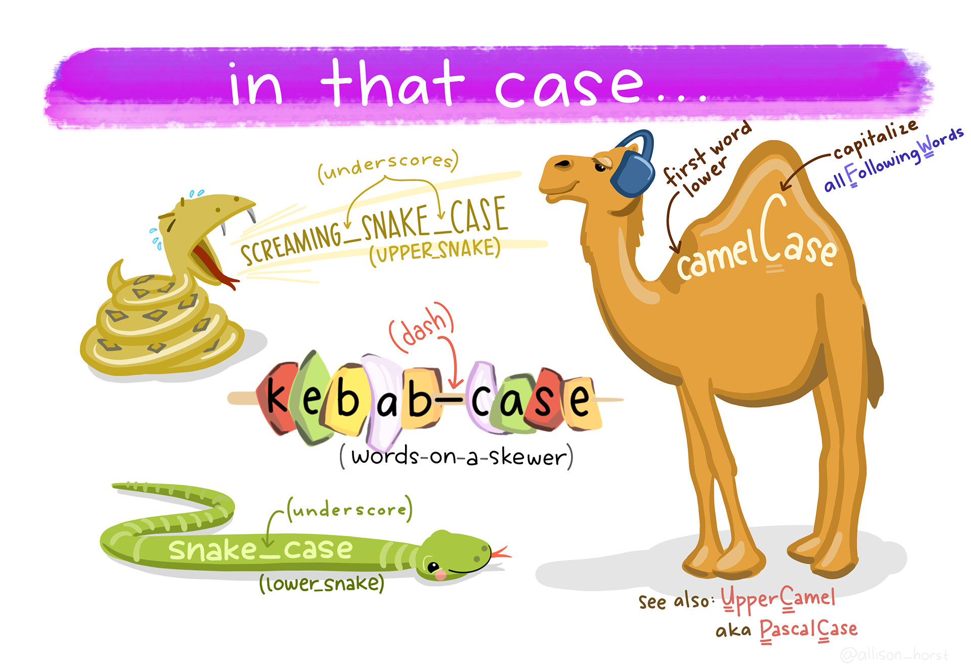
14.2.2 Three common naming styles

You will see these everywhere:

• camelCase (meanDepth)
• PascalCase (MeanDepth)
• snake_case (mean_depth)

In this course, we will default to snake_case for variables and files. This is strongly recommended for analysis scripts.

From Allison Horst. Cartoon representations of common cases in coding. A snake screams “SCREAMING_SNAKE_CASE” into the face of a camel (wearing ear muffs) with “camelCase” written along its back. Vegetables on a skewer spell out “kebab-case” (words on a skewer). A mellow, happy looking snake has text “snake_case” along it.

14.2.3 General guidelines (the “please don’t make future you angry” list)

These are simple rules that prevent a shocking number of problems:

Rule	Why it matters	Example of poor form
Avoid blank spaces	Spaces complicate coding and break formulas, file paths, and scripting	Mean Depth, Site Name, Final Data.csv
Omit special symbols like ?, $, *, +, #, (, ), -, /, }, {, |, >, <, etc.	Many special characters are treated as operators or commands in R, so using them in names can break code or make it harder to work with.	mass(g), count#, Y/N?, depth>10
Use _ as a separator	Underscores are safe, readable, and standard	mean-depth, mean.depth, mean depth
Do not begin names with numbers	Names starting with numbers are invalid or confusing in R	100m_depth, 2023_data
Make names unique	Non-unique names cause overwriting and ambiguity	data, data2, final, final_final
Be consistent with case	R is case-sensitive; inconsistency causes silent bugs	Depth, depth, DEPTH in same project
Avoid blank rows in data	Blank rows can be misread as data or missing values	Empty rows between observations in CSV
Remove comments from data files	Comments belong in scripts or metadata, not raw data	# measured in June inside a CSV
Define and document NA values	Ambiguous missing values lead to incorrect analyses	Mixing NA, 0, -999, . without explanation
Use clear, documented date formats	Ambiguous dates are easy to misinterpret	03/04/21 (is this March 4 or April 3?)

14.2.4 “Bad → Good” examples for variable names

Your variable names should be: - readable at a glance - easy to type - consistent across files and projects

Here are examples aligned with the tidyverse style guide (Hadley Wickham):

A quick translation rule:

• Use units as suffixes: depth_cm, mass_g, distance_m (do not use parentheses around units)
• Use clear boolean names: yes_no or better: is_adult, has_nest
• Prefer meaning over brevity: percentile_50 beats p50 (unless p50 is a defined term in your field)

14.3 Naming conventions for folders (project structure)

14.3.1 Why folder names matter

A good folder structure makes it hard to lose track of: - raw versus processed data - inputs versus outputs - code versus results - files that you can re-create versus ones you cannot (i.e. that you should never overwrite)

In this course, we care about reproducibility, which means: - raw data is always treated as read-only - processed data is created by scripts, acting on raw data, and never manually edited - results are generated by scripts and never manually edited

TipA folder structure that scales

A simple, stable structure (example):

• data/
  • raw_data/ (never edited)
  • processed_data/ (created by scripts)
• r_scripts/ (functions + helpers)
• analysis/ (analysis note / exercises )
• outputs/
  • figures/
  • tables/

Folder naming rules (same spirit as variable naming): - lowercase (snake_case) - no spaces - prefer underscores - descriptive names over clever names

14.4 Conventions for legible and consistent R code

14.4.1 Why code style matters

Code style is not about being fancy. It’s about making your thinking legible.

Good style: - reduces bugs - improves peer review (including lab mates and future you) - makes it easier to modify models without breaking things

NoteTwo extremely useful packages for checking R code formatting

• lintr checks your code for style problems (like a spellcheck for R code).
• styler automatically formats your code to match a consistent style.

14.4.2 “Bad → Good” examples for R code and files

These examples follow the tidyverse style guide (Hadley Wickham):

Bad	Why was it bad?	Good
Fit models.r	Contains spaces; inconsistent casing; harder to reference in code	fit_models.R
##########	No semantic meaning; comments should describe intent, not fill space	# extract elevation -----
findat	Vague name; gives no clue about content or structure	findat_mat
findat_mat	Redundant and unclear; does not describe what the matrix contains	mass_mat

A few rules we will use repeatedly:

14.4.3 Use nouns for objects and verbs for functions

• Objects (things): pufferi, pufferi_clean, model_gam
• Functions (actions): clean_data(), fit_model(), plot_effects()

14.4.4 Make “intermediate objects” obvious

If an object is temporary, label it like it is: - *_raw, *_clean, *_long, *_wide, *_summary

14.4.5 Prefer readable code over clever code

NoteOver-piped, confusing code

summary_df <-
  raw_df |>
  dplyr::filter(!is.na(count), year >= 2015) |>
  dplyr::group_by(site, species) |>
  dplyr::summarise(
    mean_count = mean(count),
    sd_count   = sd(count),
    n          = dplyr::n(),
    .groups = "drop"
  ) |>
  dplyr::filter(n >= 5) |>
  dplyr::mutate(
    cv = sd_count / mean_count,
    log_mean = log(mean_count)
  ) |>
  dplyr::arrange(dplyr::desc(log_mean))

NoteLonger but readable code

# Step 1: keep valid observations from recent years
df_filtered <- raw_df |>
  dplyr::filter(!is.na(count), year >= 2015)

# Step 2: summarize counts by site and species
df_summary <- df_filtered |>
  dplyr::group_by(site, species) |>
  dplyr::summarise(
    mean_count = mean(count),
    sd_count   = sd(count),
    n          = dplyr::n(),
    .groups = "drop"
  )

# Step 3: retain well-sampled groups
df_sufficient <- df_summary |>
  dplyr::filter(n >= 5)

# Step 4: compute derived metrics
df_metrics <- df_sufficient |>
  dplyr::mutate(
    cv       = sd_count / mean_count,
    log_mean = log(mean_count)
  )

# Step 5: order results for inspection
summary_df <- df_metrics |>
  dplyr::arrange(dplyr::desc(log_mean))

14.4.6 A final note about reproducible analyses

In workflow tools like targets, names are not simply cosmetic. They define nodes in a dependency graph (i.e. the ways all your inputs, processes, and outputs are connected). If names are unclear, the graph is unclear. If the graph is unclear, the workflow is not reproducible.

TipPractical guidance

• Use CSV/TSV when the dataset is small enough to load quickly and inspect easily.
• Consider .RDS when you want an R-native format that preserves object structure.
• Consider .parquet when files get big and you care about speed + file size.

---

14.5 Your “minimum standard” checklist (use this before you submit anything)

NoteNaming + style checklist

Data + variables

• Column names are snake_case
• No spaces or special characters in column names
• Units are explicit where relevant (_m, _cm, _g, _s)
• Missing values are documented (what is NA, what is 0, what is “not observed”?)
• Dates are in a clear, documented format (and the order is not ambiguous)

Folders + files

• Folder names are lowercase and descriptive
• Raw data are not edited in place
• Processed data are created by scripts (not by hand)

R code

• Objects use nouns; functions use verbs
• Scripts are readable (spacing, line breaks, consistent naming)
• You can restart R and run the workflow without relying on “things in memory”

14.6 Practice task (recommended)

1. Pick one of your current projects (or a past project).
2. Rename:
   • 5 confusing variables
   • 3 confusing files
   • 1 confusing folder
3. Make one small style improvement:
   • consistent naming
   • readable comments
   • break one long chunk into 2–3 meaningful steps

The goal is not perfection. The goal is to start practicing now.