m_ri <- glmmTMB(
  y ~ time + (1 | plot_id),
  data = dat,
  family = poisson
)27 GLMM epilogue
27.1 Random slopes and intercepts
Before fitting a mixed-effects model, your task is to decide how group-level variation is included in your model. You can ask yourself two distinct questions:
- Do groups differ only in their average response (random intercepts)?
- Do groups respond to predictors (random slopes)?
Consider this example: You are studying seasonal changes in foraging activity of arctic jackalopes across multiple tundra plots. Each plot is surveyed repeatedly over time to measure how average feeding rate changes throughout the breeding season.
With this study in mind, we now must decide how variation among plots should be characterized in the model. Two common random-effects structures differ in whether plots vary only in their baseline activity or also in how their activity changes over time. This kind of decision should be anchored in your primary hypotheses and your own expert knowledge.
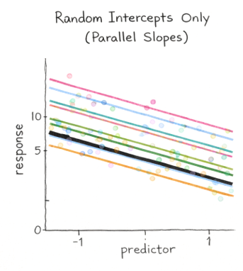
NoteRandom intercepts (constant slopes)
Logic: Each group gets its own baseline level (intercept), but the effect of timeis assumed to be the same in every plot (one common slope)
glmmTMB notation: Use (1 | plot_id) (or equivalently (time | plot_id) only if you intend random slopes too; see next box).
Model structure in glmmTMB:
Key point: Time appears as a fixed effect (y ~ time + ...) because the population-level time trend is estimated once for everyone; plots only shift up/down via their random intercepts. If you were not interested in estimating an effect size for time, then that term could be easily omitted.
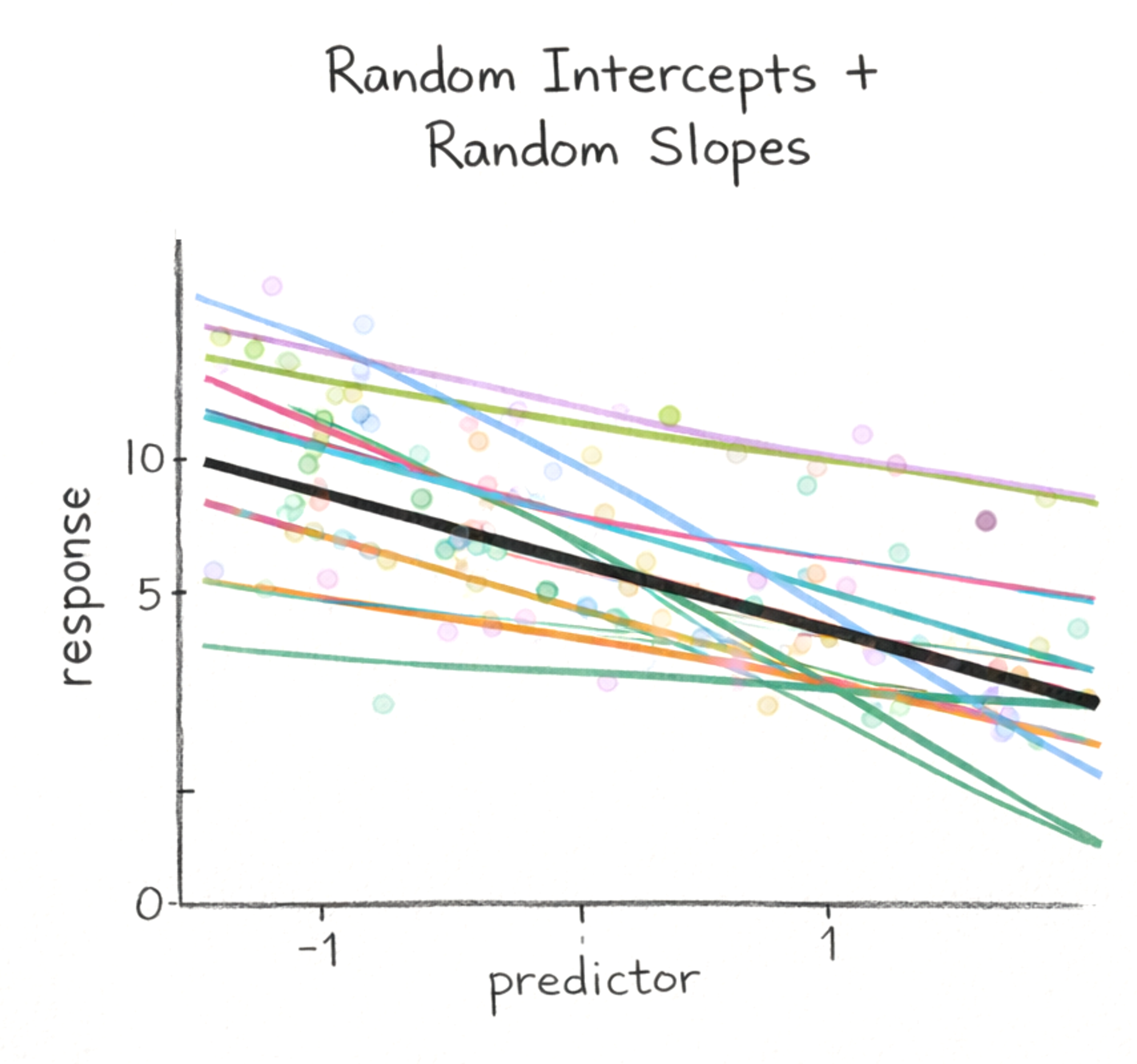
NoteRandom slopes and intercepts
Logic: Each group gets its own baseline level (intercept) and its own effect of time (slope). In other words, groups can start at different levels and change at different rates over time.
glmmTMB notation: Use (time | plot_id), which expands to (1 + time | plot_id) (random intercept + random slope, with their correlation estimated by default).
Model structure in glmmTMB:
m_ris <- glmmTMB(
  y ~ time + (time | plot_id),
  data = dat,
  family = poisson
)
Key point: Time must still appear as a fixed effect (y ~ time + ...) because the model estimates the overall population-level time trend. The random slope allows each group to deviate from that overall trend, rather than replacing it. Because time is in the random effects structure, time also is required to be in the fixed-effects portion.
27.2 Should you remove random effects that explain no variance?
This question comes up repeatedly, and it usually gets framed as a choice between two approaches:
- Leave the random effect in
- Take the random effect out…and then justify it
Option A: Leave the random effect in Usually If the study design dictates the random effects structure, then keep it. If the grouping variable reflects real clustering in the data, that structure should be modeled.
If the estimated variance is near zero, retaining the random effect typically does no harm. It simply indicates that little variation is attributed to that level. The model remains consistent with the design.
Option B: Remove the random effect and justify it The second option is to compare models with and without the random effect using a formal statistical approach. However, even if you use such an approach, you need to carefully justify your decision. Possible approaches included likelihood-ratio tests (LRTs) using Maximum Likelihood, where you show the statistical comparison and then explain why the simpler model improves the fit.
There is no clear answer as to whether you should remove a random effect if it explains no variance. A random effect is usually a design issue (e.g. blocking effects, nested units of sampling). Inclusion of the random effect should come naturally from the structure of your study.
TipPractical note: removal of random effect
From a design perspective, it is often safer to retain structure that was motivated by your knowledge of ecology/biology. Therefore, I strongly suggest removing random effects (or levels within a hierarchical random effet) if and only if your model fails to converge. Otherwise, leave them in; there is no harm in doing so.
27.3 How many levels are required?
How many levels of a random effect (e.g. two sites) must exist in order for a random effect to be considered for inclusion in the model. This is a perennial question. Scientists are attracted to rules. Yet, there is not one. In the literature, in lab discussions, and in online statistics forums, you will hear and read claims about the minimum number of allowable levels for a random effect: 4, 5, 6, or, in one case I read long ago, even 14 levels(!). At minimum, the varied opinions suggest that there is no consensus. The fundamental point here is very simple:
There is no strict minimum number of levels that dictates inclusion of a random effect.
As the number of levels of a random effect decreases, the mixed model approaches the same form as a standard GLM. There is nothing special that happens at three, four, or five levels. That is, a model does not suddenly become invalid below some arbitrary cutoff (just as nothing special happens at p=0.05 versus p=0.51) With very few levels, a random effect may add little extra information to the overall model. But including the random effect does not harm the analysis. Even small variance components can improve inference by accounting for clustering and non-independence. And that is a win for science.
If the data are clustered, model the clustering. Do not rely on arbitrary rules. Use your knowledge about the natural structure of your dataset. To help you bolster your argument, you can read Gomes, D.G.E. (2022).
27.4 How should my dataset look in a spreadsheet?
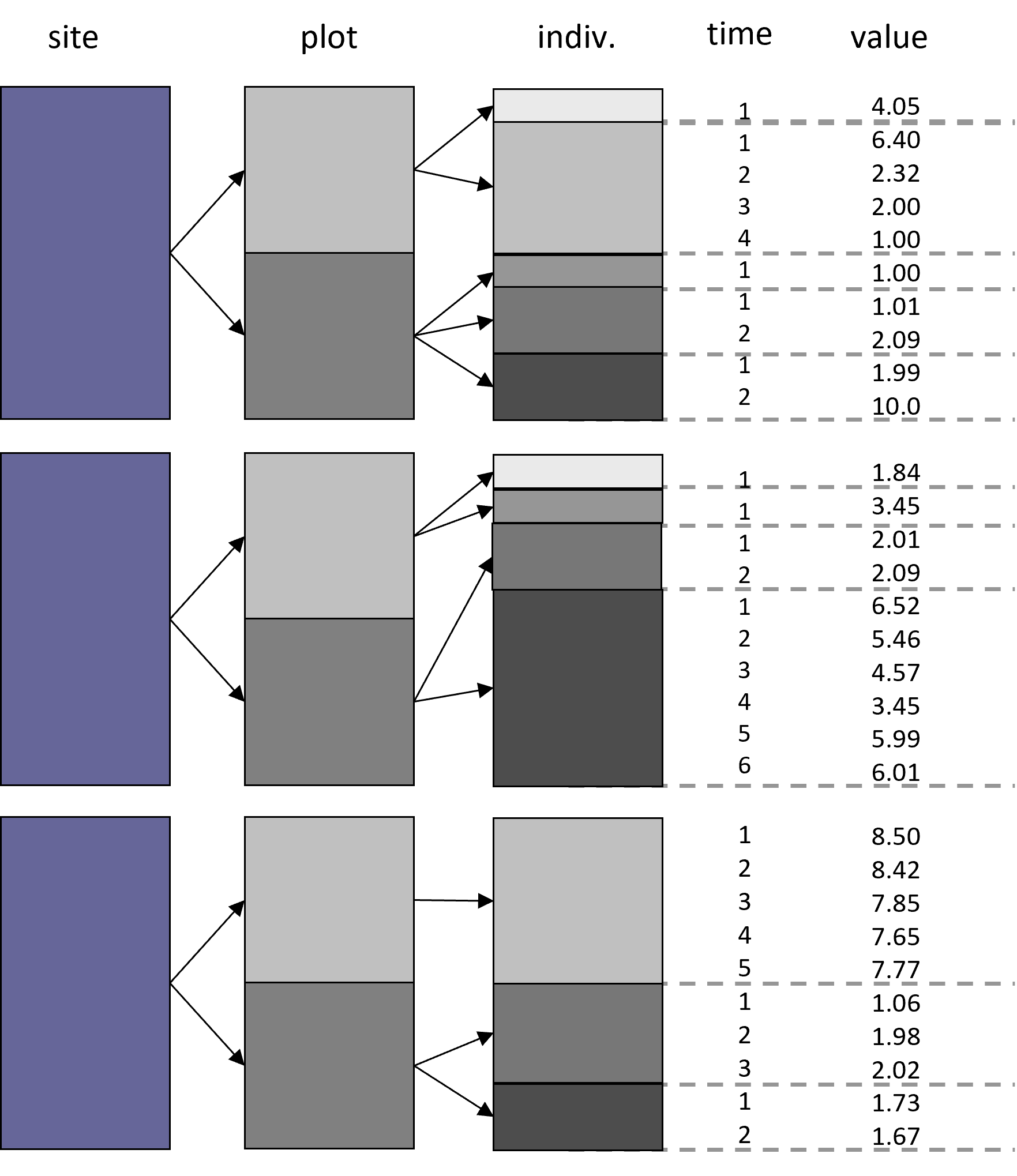
With all this talk of what random effects are, we sometimes forgot to ask about how these can be formatted. Random effects are simply grouping variables; they are simply different variables (columns) of your dataset. Below is a stylized version of how this might look generally. This represents n=30 rows of data in a spreadsheet.
Measurements in the stylized spreadsheet at right were collected at different times for 12 individuals within 6 plots, which were split between three sites. Site 1 (top blue box) had six individuals; Site 2 (middle blue box) had four individuals; Site 3 (bottom blue box) had three individuals.Dotted lines delineate different individuals’ data points across time. Data are severely unbalanced. Arrows between boxes in site, plot, and individual indicated how small grouping levels are nested within larger ones.