source("chapters/class_r_scripts/load_packages.r")21 GLM Introduction
21.1 Separating signal from noise
Our task as scientists is to learn how to separate the patterns that carry meaningful information (signal) from the variation that does not (noise). This is why we use all of these silly models in the first place. So, what exactly are models?
Models are hypotheses about how the data were generated.
21.1.1 Comparing GLMs to vintage models (ANOVAs and t-tests)
Let us begin this introduction to our primary modeling framework (the GLM) by comparing GLMs to some familiar statistical approaches.
Here, we provide some simulation code that will (hopefully) convince you that GLMs are pretty much the same kinds of models that you were exposed to in your introductory statistics courses back in the day. As you will quickly see, however, GLMs are highly flexible and will allow you to extract the maximum amount of signal from your noisy data.
We will simulate a fake dataset that has two groups (1 and 2). The values for each group follow normal distributions with a standard deviation of 1. The groups differ in their mean values, however, by one unit.
set.seed(100) # this is a random seed that ensures example reproducibility
nval <- 50 # Generate some fake data
group1 <- rnorm(nval, mean=5, sd=1)
group2 <- rnorm(nval, mean=6, sd=1)
d <- data.frame(id=rep(c("group1", "group2"), each=nval),
  y=c(group1, group2))
p <- ggplot(d, aes(x = id, y = y, fill = id)) +
geom_boxplot(width = 0.6, outlier.alpha = 0.5) +
labs(
x = "Group ID",
y = "Response"
) +
theme_minimal(base_size = 14) +
theme(
axis.title = element_text(size = 16),
axis.text = element_text(size = 14)
) +
guides(fill = "none") # hide legend if redundant
p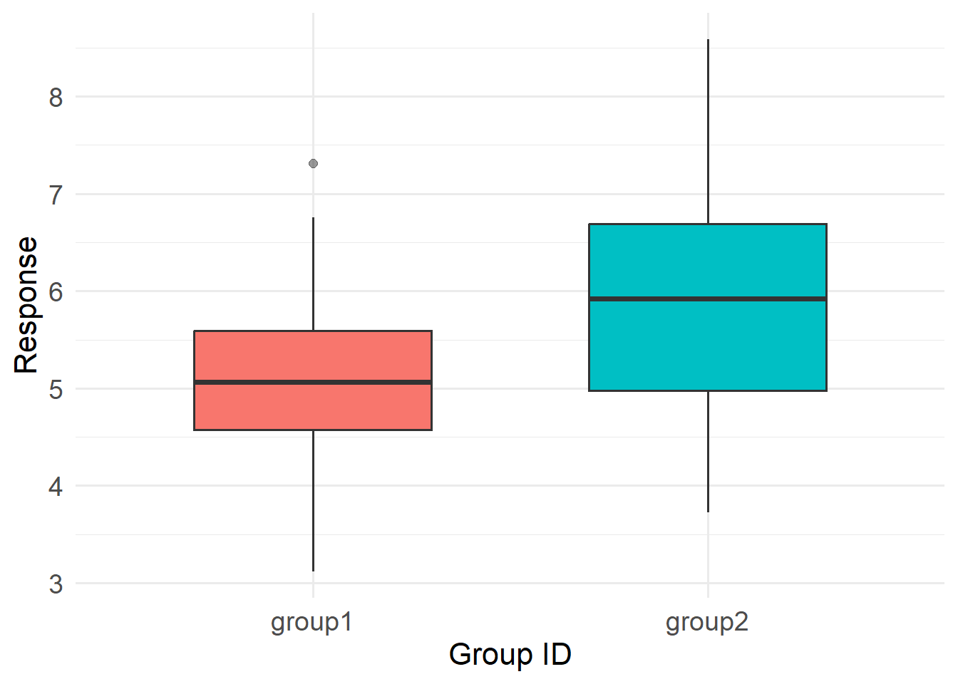
Now, using three models (t-test, ANOVA, and GLM), let us test the hypothesis that these two groups differ. Remember that t-tests and ANOVAs are linear models that assume, among other things, that both the signal and the noise follow a Gaussian/Normal distribution. Note that we need to convert the ANOVA’s F-stat to a t-statistic for comparability. You can see the code for this multi-model comparison in this callout box:
You can see that all of the t-values are exactly the same (t = 4.119985). Fantastic! Now you can sit back and silently reconsider your desire to use a t-test or ANOVA (or anything similar). Let us say that we are not abandoning t-tests and ANOVAs; instead, we are outgrowing them. The table below shows a number of other advantages that GLMs have.
| Functionality / Capability | t-test | ANOVA | GLM |
|---|---|---|---|
| Unbalanced sample | ✅ | ✅ | ✅ |
| Compare more than two groups | ✅ | ✅ | |
| Handle continuous predictors | ✅ | ||
| Handle non-Normal distributions | ✅ | ||
| Complex hierarchical random effects | ✅ | ||
| Use link functions (log, logit, etc.) | ✅ | ||
| Predicted values from model output | ✅ | ||
| Nonlinear extensions | ✅ | ||
| Under current development | ✅ |
Hopefully, this short exercise convinces you that GLMs and their extensions (Generalized Linear –and Additive– Mixed Models) no longer need to be viewed as “advanced statistics”; they can simply be used as a formal and unified language for ecological thinking.
21.1.2 Setting the stage for GLMs
Most textbook treatments of GLMs start off examining a model with Gaussian (normally distributed) errors. The Gaussian models have core assumptions that are likely familiar and comfortable to most of you, including:
- The response variable is continuous
- The residual variance is constant (homoscedastic)
- The error distribution is symmetric
- The outcome can take any real value (including negatives)
In many classroom situations, that works beautifully. If we are modeling body mass of adults (why adults?), temperature, or some other roughly symmetric continuous variable, the Gaussian/normal distribution is often appropriate. However, the Gaussian/normal distribution is often the exception rather than the rule because:
Most ecological data are not normally distributed.
Why? As ecologists, we regularly collect data on proportions, rates, skewed measurements, zero-heavy processes, and, perhaps most commonly, counts like:
- Number of individuals observed
- Number of detections on a recorder
- Number of nests in a plot
- Number of disease cases
For example, consider counts of events. Count distributions –often best approximated by a Poisson distribution– have their own features, including:
- Values cannot be negative.
- Values are discrete (not continuous)
- They often have variances that equal or increase with their mean
- They are frequently right-skewed
A Gaussian model, on the other hand, ignores almost everything about how most ecological data are generated. Therefore, in this section, we will first explore the Poisson GLM, which is designed specifically for count data. It:
- Restricts predictions to non-negative values.
- Allows variance to increase with the mean.
Furthermore, using a Poisson GLM allows you to see the internal architecture of a GLM. It is a bit more difficult to see how a GLM works when using a Gaussian distribution. In a Poisson GLM, the GLM components are clearly delineated:
- The error distribution describes the noise.
- The linear predictor describes the signal.
- The link function connects the expected value of the response to the linear predictor
Because those parts are visibly distinct, the Poisson model makes it much easier to understand what a GLM is actually doing.
21.2 The Poisson GLM: Model Specification
At first glance, especially if you have had no formal mathematical training, the formal notation of a GLM can appear very intimidating. Symbols such as \(Y_i\), \(\mu_i\), and \(\eta_i\) may give the impression that the model is mathematically difficult to the average scientist. In reality, these equations simply provide an efficient way to describe simple concepts about data and model structure. Fundamentally, a relatively small set of equations can describe:
- How observations in a dataset vary
- How predictors influence expected responses
- How effects are linked to observable data
Writing the mathematical form of a model really does helps demystify it. At least, that will be my attempt in this course. Each component of how we mathematically formalize a GLM corresponds to one part of the data-generating process.
First, we begin with our observations (our dataset). Using each observation \(i\) and sample size \(n\), we define our dataset as: \(i = 1, \dots, n\):
We then set up the three core components of our GLM:
21.2.1 Random Component (Noise)
The random component –the unmeasured structure of your model– is formalized as:
\(Y_i \sim \text{Poisson}(\mu_i)\), where:
- \(Y_i\): observed count for observation \(i\)
- \(\mu_i\): expected (mean) count for observation \(i\)
Recall that a Poisson distribution has a mean and variance that are equal: the expected count is \(\mu_i\), and the variability around that expectation is also \(\mu_i\). This means that as the expected number of events (counts) increases, the spread of the data increases proportionally, so larger means naturally are associated with greater variability.
\(E(Y_i) = \mu_i\) \(\text{Var}(Y_i) = \mu_i\)
The notation \(Y_i \sim \text{Poisson}(\mu_i)\) simply states:
The observed count \(Y_i\) is a random draw from a Poisson distribution with mean \(\mu_i\).
There is nothing mystical in this expression. It formalizes three important ideas:
- The outcome is a count (non-negative integers only).
- The mean and variance are equal.
- Variability scales with the expected value.
By writing the distribution explicitly, we clarify:
- What values are possible
- How uncertainty behaves
- How variance depends on the mean
The equation prevents hidden assumptions. Without it, readers might assume constant variance or continuous outcomes. The formal notation makes those assumptions transparent. So, I strongly encourage you to take some time and get comfortable writing out your models in this way. These points will be reiterated below in the link function section.
21.2.2 Systematic Component (Signal)
\(\eta_i = \beta_0 + \beta_1 X_i\)
Definitions
- \(\eta_i\): linear predictor
- \(\beta_0\): intercept
- \(\beta_1\): slope parameter
- \(X_i\): predictor value for observation \(i\)
This expression is simply a linear equation. It states:
The structured component of the model is a straight-line function of the predictor.
There is no randomness here. If \(X_i\) and the coefficients are known, \(\eta_i\) is determined exactly. The equation clarifies:
- How predictors are assumed to influence outcomes.
- That effects are additive on the linear predictor scale.
- That the relationship is directional and structured.
Without writing this formally, it is easy to obscure how predictors fold into the model. The mathematical form adds clarity about what is signal and what is noise.
21.2.3 Link Function
The final component of a GLM is the link function, and its role is more conceptual than technical. It connects the structured part of the model (the signal) to the distribution that governs randomness (the noise).
In a GLM, the variance is defined as a function of the mean; this is general to any GLM. Recall that, in a Poisson model:
\(E(Y_i) = \mu_i\) \(\text{Var}(Y_i) = \mu_i\)
This tells us something very cool: once the mean \(\mu_i\) is determined, the amount of variability is determined as well. The expected value and the noise structure are mathematically tied together. The link function is simply the bridge between signal and noise. It takes the output of the linear predictor (the signal) and converts it into the mean of the response distribution. Because the variance depends on that mean, the signal indirectly determines the scale of the noise.
Put another way, we first build a straight-line equation:
\(\eta_i = \beta_0 + \beta_1 X_i\)
We then transform that linear result to obtain a valid mean:
\(\mu_i = \exp(\eta_i)\)
That exponentiation is all the link function is:
a rule that converts the output of the linear predictor into a proper mean for the distribution. Since the variance depends on the mean, this transformation also determines how much noise we expect.
21.3 Summary: the compact form of a Poisson GLM
Let us put this all together in a single structure that could be included in a scientific paper:
\(Y_i \sim \text{Poisson}(\mu_i)\)
\(\log(\mu_i) = \beta_0 + \beta_1 X_i\)
This compact form contains the entire model. When broken apart, it describes:
- The distribution of variability (the Poisson portion)
- The structured influence of predictors (the line equation)
- The transformation connecting structure to expectation (the log operator)
The mathematical notation is far more concise than what we sometimes see in the articles’ descriptions of statistical analyses. The concise form communicates all of the components of the model in a straightforward way. The value of writing them formally is not useless abstraction; it is clarity about how our decisions are translated into strong inference.
21.4 Testing yourself: thinking about signal and noise in a totally real dataset
For this conceptual self-test, we will use a dataset that was collected from a population of Lepusantilocapra pufferi (puffer jackalope) starting in the mid-1970s.
You will need the following file (simply click to save):
The data include the following variables:
site: where the individuals were sampledabund: number of individuals detected at each locationdens: density of individuals at each sampling locationmean_depth: mean depth, in meters of the sampling locationyear: year of the studyperiod: 1=before and 2= after introduction of Pelicanus pufferivorus (puffer-jackalope pelican)x_km: longitude (decimal degrees) of sampling locationy_km: latitude (decimal degrees) of sampling locationswept_area: size in square meters of the sampling location (effort)
Familiarize yourself with these data (especially mean_depth, dens, and abund) and then think about the following questions. Click to expand each box for the answer.